Achieve a smooth and precise pick & place through PID tuning
| Site: | NiryoAcademy |
| Course: | PID Tuning for a Pick & Place |
| Book: | Achieve a smooth and precise pick & place through PID tuning |
| Printed by: | Guest user |
| Date: | Monday, 20 October 2025, 7:15 PM |
Introduction
Objective: understand the influence of the gains P, I, and D on the response of axis 5 and achieve precise, fast, and oscillation-free motion.
Prerequisites
- NiryoStudio installed and connected to the Ned2.
- Access to the PID module.
- An obstacle-free area for axis 5 movements.
Learning Outcomes
- Interpret setpoint / actual / error plots.
- Tune P, I, D to meet dynamic criteria (speed, overshoot, stability).
- Implement a structured experimental approach.
PID Tuning of Axis 5
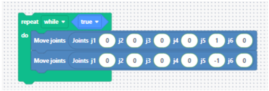
1) Create a test program (Blockly)
Move axis 5 between two angles (e.g., −1.0 rad ↔ +1.0 rad). Create a Blockly program and name it “PID_tuning”.
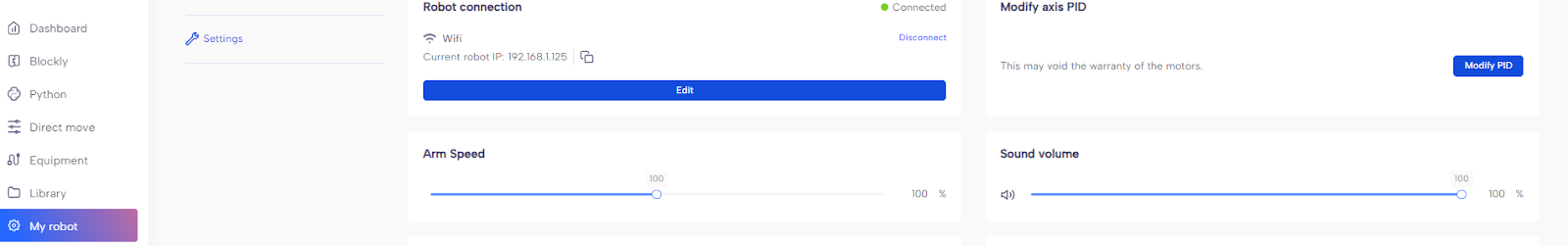
2) Open the PID parameters
In NiryoStudio: My Robot → Settings → Edit PID.
Adjust the gains P, then I, then D. After each change, run the PID_tuning program and observe the plots.
3) What to look for on the plots?
- Speed (rise time) without overshoot.
- Fast stabilization (error → 0).
- No oscillations or visible vibrations.
Example configurations (theoretical)
| P | I | D | Type | Observed behavior |
|---|---|---|---|---|
| 1200 | 400 | 300 | ✅ Stable | Balanced motion |
| 800 | 700 | 200 | ✅ Stable | Accurate, but slow response |
| 2500 | 1000 | 0 | ⚠️ Unstable | Overshoot, oscillations |
| 100 | 2000 | 0 | ⚠️ Unstable | Integral windup, delayed response |
| 3000 | 0 | 0 | ⚠️ Unstable | Purely proportional response, abrupt jumps |
⚠️ These values are indicative for analysis. Each load may require adjustment.
Guided interpretation of tests
Test on gain P
Configuration: P = 3000, I = 0, D = 0.
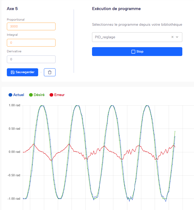
In this test, the proportional gain (P) was significantly increased to 3000, while the integral (I) and derivative (D) gains were set to zero. The blue curve (actual position) closely follows the green curve (desired command), with a relatively small and stable red curve (error). This shows that the system reacts quickly to deviations.
However, a high P value often causes instability or visible shaking, especially in real mechanical systems. Even if it is not obvious on the graph, in practice one can observe vibrations or jerky movements, as the robot corrects even the smallest error too aggressively. Therefore, it is crucial to find a compromise: a P high enough to follow the command properly, but not so high that it triggers overreactions.
Test on gain I
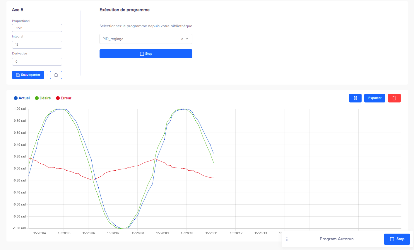
Configuration: P = 200, I = 1200, D = 0.
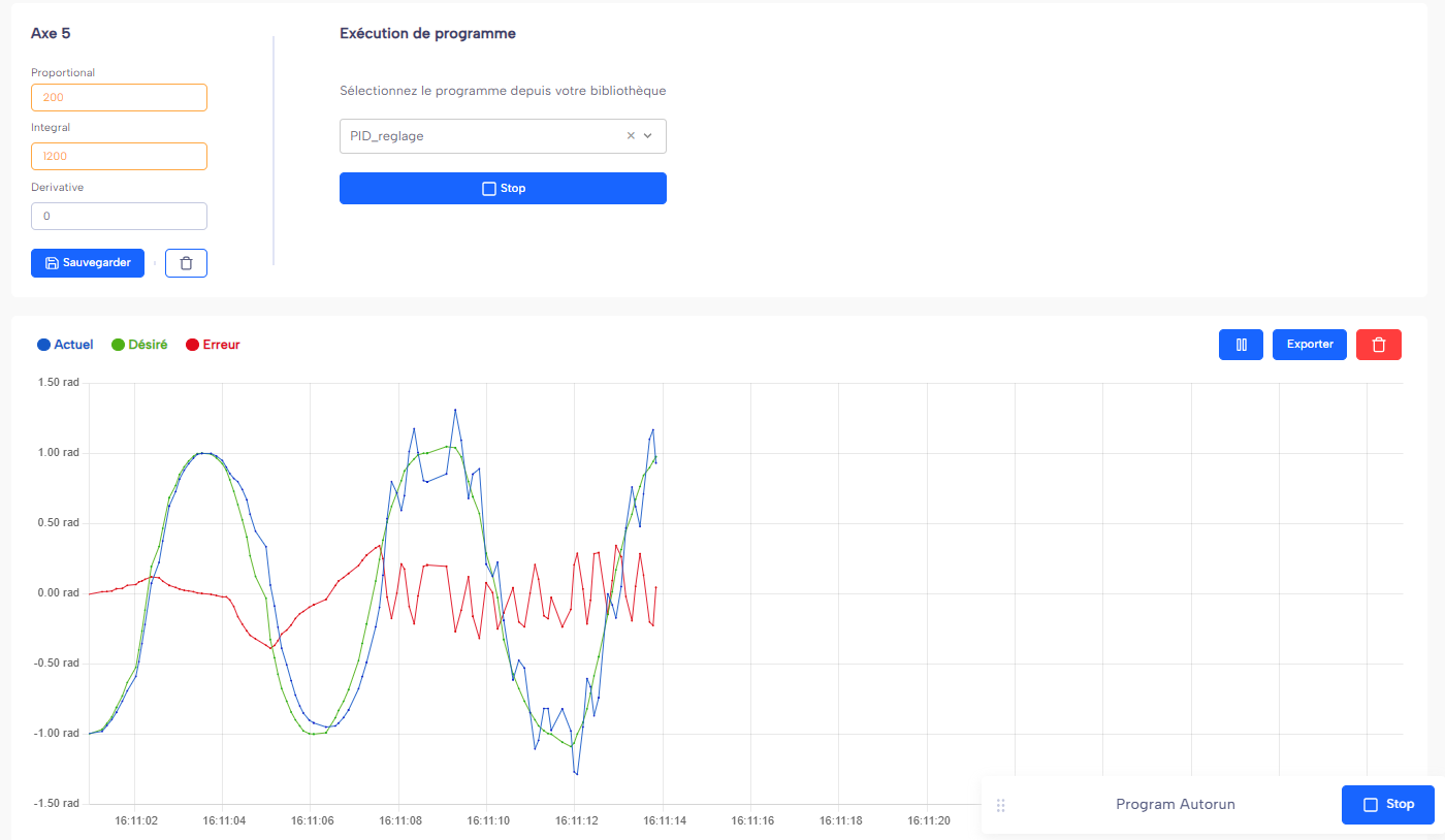
In this example, the integral gain (I) was significantly increased to 1200, while the proportional gain (P) was reduced to 200, and the derivative (D) remained at zero. The red curve representing the error becomes persistent and oscillates around a non-zero value. This occurs because the integral term accumulates the error over time; if too large, it can create slow oscillations or instability. The system takes longer to follow the desired command (green curve), and the gap with the actual position (blue curve) remains visible, especially during direction changes.
Test on gain D
Configuration: P = 100, I = 0, D = 3000.
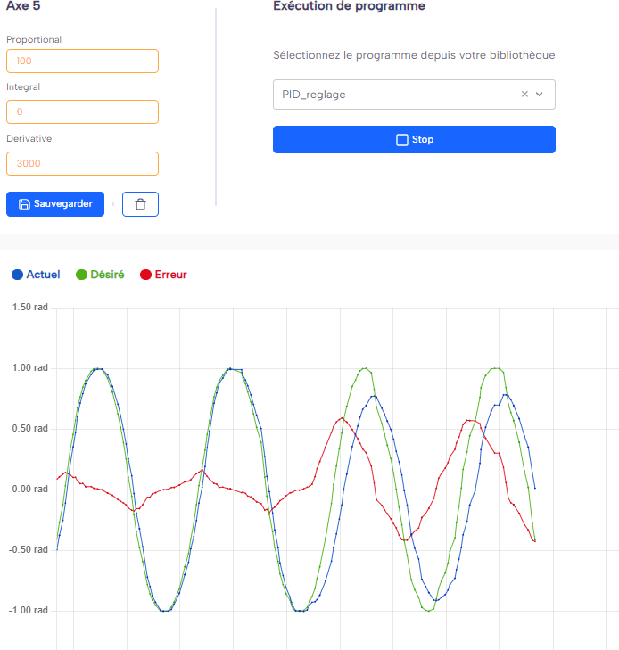
Here, a change in parameters was made during motion: the derivative gain (D) was strongly increased to 3000, while the proportional gain (P) was reduced to 100. This configuration causes a noticeable delay between the blue curve (desired command) and the green curve (actual axis position). This delay indicates a slower response, increasing the error between the command and the reached position.
Interpretation memo
- P ↑ → faster response, but risk of overshoot or oscillations.
- I ↑ → eliminates static error, but may cause windup.
- D ↑ → reduces overshoot, but slows down response.
Your mission: reach clear criteria
- A fast motion without overshoot.
- Quick stabilization (error → 0 in a short time).
- No visible oscillations or vibrations.
Suggested tuning procedure (heuristic):
- Start with
P ≈ medium,I = 0,D = 0. Increase P until the first oscillations appear, then reduce it by ~10–20%. - Add a small amount of D to eliminate overshoot and stabilize.
- Gradually introduce I to remove residual error, while watching for windup.
- Repeat the tests (PID_tuning program) and compare the curves.
Common pitfalls
- P too high → vibrations, noise, overcorrections.
- I too high → slow response + slow oscillations (windup).
- D too high → sluggish response, noticeable delay.
Practical tips
- Keep a log of tested values (P, I, D) + screenshots of the curves.
- Always test with the same sequence of angles/speed to compare accurately.
- Payload and friction influence tuning → adjust the gains accordingly.
Restore factory parameters
If needed, you can restore the default PID parameters provided by the manufacturer to return to a stable baseline behavior.
Pick & Place Challenge
Objective: program a pick & place sequence and obtain a wrist movement (axis 5) that is smooth, stable, and free of jerks during object placement.
Challenge to program
- The robot picks up an object at the pickup position.
- It places the object at position 1 with a specific wrist orientation.
- It returns to the pickup position and grabs another object.
- It places this second object at position 2 (possibly with a different orientation).
Example sequence
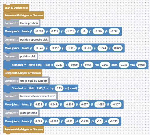
💡 Adjust j5 in your blocks/poses to set a clear orientation and observe the impact of PID parameters.
Visualize & analyze the curves
Run the sequence while displaying the plots for each motion in NiryoStudio’s PID module:
- Setpoint (axis 5 position reference)
- Actual (measured position)
- Error = setpoint − actual
Criteria to achieve
- No significant error spikes (especially during placement).
- Fast convergence of the actual position to the setpoint.
- Smooth, stable, and jerk-free wrist motion.
Example configurations (pick & place)
⚠️ Example values that clearly show the effects of each gain during a pick & place, without using extreme cases:
| P | I | D | Type | Observed behavior |
|---|---|---|---|---|
| 2000 | 0 | 0 | ⚠️ Unstable | Vibrations |
| 200 | 1200 | 0 | ⚠️ Unstable | Jerky movements |
| 100 | 0 | 3000 | ⚠️ Unstable | Axis 5 response too slow |
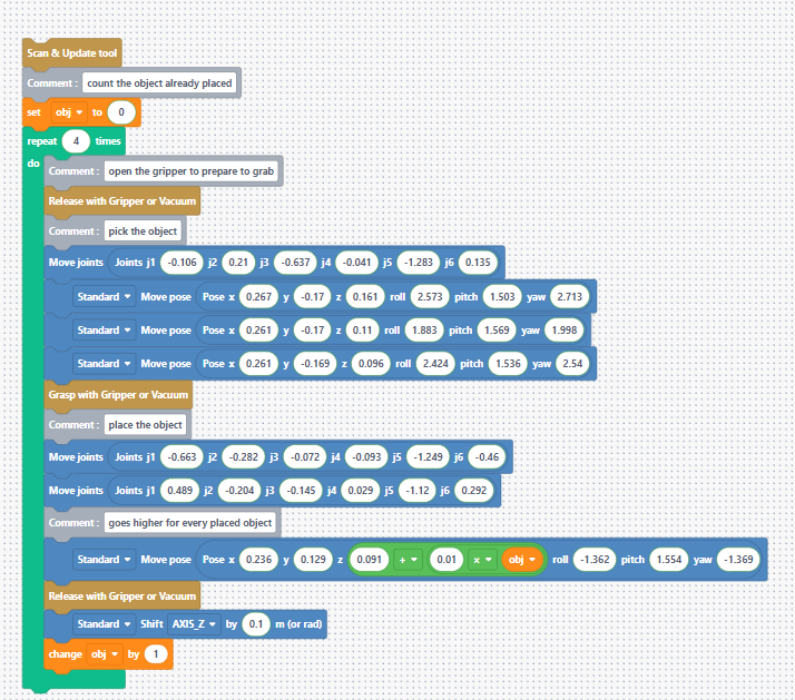
Activity BONUS
Stack the objects on top of each other to form a stable tower. It’s up to you to tune the PID so that the tower doesn’t collapse during manipulation!
For this example, we use the objects provided with the vision kit, each having a thickness of 1 cm. Therefore, we added 0.01 m to the Z value after placing each object.
What are the effects of each gain?
Proportional Gain (P)
The proportional term produces an output directly proportional to the current error. The farther the system is from the target, the stronger the correction.
When the proportional gain is increased, the system reacts faster and the rise time decreases. However, if the value is too high, it may cause overshoot and oscillations.
Reducing the proportional gain leads to a slower, less responsive reaction. In some cases, the system may never fully reach the target, resulting in a steady-state error.
A good analogy is a spring pulling the system toward its target: the farther it is, the greater the restoring force.
Integral Gain (I)
The integral term accumulates past errors over time. Its goal is to eliminate steady-state error, i.e., when the system remains near the target without ever fully reaching it.
Increasing the integral gain improves long-term accuracy and allows the system to reach the target precisely. However, if the gain is too high, it can cause overshoot, slow response, and a phenomenon called windup—when the output becomes excessively large due to accumulated error.
Reducing the integral gain may leave a steady-state error, but the system becomes more stable and less prone to abrupt corrections.
You can think of this term as a memory: the controller says, “I’ve been off target for too long, I need to push harder.”
Derivative Gain (D)
The derivative term considers the rate at which the error changes. It acts like a brake, slowing the system as it approaches the target by anticipating future error.
Increasing the derivative gain helps reduce overshoot and dampens oscillations, making the system more stable. However, if it’s too high, it can make the response slow or overly sensitive to sensor noise.
Reducing the derivative gain decreases damping, which may lead to instability and increased overshoot.
This term smooths the approach to the target, like gradually braking before coming to a stop.
Summary Table:
|
Gain |
General Effect |
Too Low → |
Too High → |
|
P |
Quick reaction to error |
Slow response, persistent error |
Overshoot, oscillations |
|
I |
Eliminates long-term error |
Steady-state error remains |
Windup, instability, overshoot |
|
D |
Dampens motion |
Oscillations, instability |
Slow response, noisy control |